
[논문리뷰] Graph Attention Networks
- 해당 논문은 Graph에 Attention을 적용하여 explainable한 graph embedding을 시도하였다.
Abstract
We present graph attention networks (GATs), novel neural network architectures that operate on graph-structured data, leveraging masked self-attentional layers to address the shortcomings of prior methods based on graph convolutions or their approximations. By stacking layers in which nodes are able to attend over their neighborhoods’ features, we enable (implicitly) specifying different weights to different nodes in a neighborhood, without requiring any kind of costly matrix operation (such as inversion) or depending on knowing the graph structure upfront. In this way, we address several key challenges of spectral-based graph neural networks simultaneously, and make our model readily applicable to inductive as well as transductive problems. Our GAT models have achieved or matched state-of-the-art results across four established transductive and inductive graph benchmarks: the Cora, Citeseer and Pubmed citation network datasets, as well as a protein- protein interaction dataset (wherein test graphs remain unseen during training).
1 Introduction
- (Background) 기존의 CNN은 grid-like structure에서 좋은 성능을 보여왔음 (e.g. image classification, semantic segmentation, machine translation, …)
- 그러나 어떤 데이터들은 grid-like structure보다는 (arbitrarily structured) graph의 형태로 구성되어 있음 (e.g. social networks, telecommunication network, biological networks, …)
- Graph 데이터는 노드 간의 순서(ordering)이 없고 구조가 매우 다양하게 형성될 수 있으며, 노드마다 이웃의 수가 너무 상이함
- CNN에서는 여러 번 layer를 쌓아 특정 부분의 정보를 요약하는 효과(increase receptive fields)가 있고, graph에서는 여러 번 layer를 쌓으면 multi-hop 정보를 반영
- (Earlier works) 그래프와 관련한 초기의 연구들은 directed acyclic graphs에 집중되었으나 GNN의 등장으로 다양한 형태의 그래프들을 다룰 수 있게 됨 (e.g. cyclic, undirected, …)
- GNN은 노드의 상태가 수렴할 때까지 반복하는 프로세스로 구성되어 있음
- input에 그래프가 들어오면 1) aggregate/message passing, 2) combine/update, 3) readout의 과정을 거쳐 output 그래프 임베딩이 형성
- 1) target-neighbor: 타겟 노드와 이웃 노드의 (k-1)th hidden state 결합; $a_v^{(k-1)}=\sum_{u \in N(v) \cup {v}} \frac{h_u^{k-1}}{\sqrt{|N(v)||N(u)|}}$
- 2) target-target: kth hidden state와 (k-1)th hidden state 결합; $h_v^{(k)}=ReLU(Wa_v^{k-1})$
- 3) total: target node마다 계산한 hidden state를 결합; $H^{(t)}=ReLU((D^{-\frac{1}{2}}(A+I)D^{-\frac{1}{2}}H^{(t-1)}W)$
- 추후에 gated recurrent units를 propagation step에 도입하기도 함
- 층을 깊게 쌓으면 over fitting이나 vanishing gradient 문제가 발생할 수 있으므로 combine 과정에서 GRU를 사용함
- GNN은 노드의 상태가 수렴할 때까지 반복하는 프로세스로 구성되어 있음
- (Earlier works) convolution을 그래프에 도입하고자 하는 시도는 spectral과 non-spectral로 구분됨
- spectral: node classification에서 성공적으로 적용됨 (Bruna et al., 2014; Henaff et al., 2015; Defferrard et al., 2016; Kipf and Welling, 2017)
- 그러나 학습된 필터는 그래프의 구조에 영향을 받는 Laplacian eigenbasis를 사용하기 때문에 특정 구조에서 학습된 모델을 다른 구조를 가진 그래프에는 적용할 수 없음 → 이 논문에서는 구조의 영향을 받지 않음
- non-spectral: convolution을 바로 그래프에 사용하여 인접 노드들에 대해서 필터 적용 (Duvenaud et al., 2015; Atwood and Towsley, 2016; Hamilton et al., 2017)
- 그러나 이웃 노드의 수를 결정하거나 CNN에서처럼 특정 property에 대한 가중치를 공유하는 것이 어려움
- GraphSAGE: 노드를 inductive하게 represent
- 1) aggregate: node별 중요도를 고려하기 위해 normalize를 해야함 + LSTM을 사용하여 neighbor 간의 순서를 고려해주어야 함 + Pooling을 사용
- 2) combine: target node와 aggregated 값을 concat하여 combine
- Transductive v.s. Inductive
- Transductive: known node와 edge를 가지고 supervised learning해서 연결된 unknown node와 edge를 predict
- Inductive: 알고 있는 graph에 대해 학습 후, 새로운 graph에 적용하여 node, edge 추정
- spectral: node classification에서 성공적으로 적용됨 (Bruna et al., 2014; Henaff et al., 2015; Defferrard et al., 2016; Kipf and Welling, 2017)
- (Earlier works) Attention: sequence-based tasks에서 많이 사용 (e.g. machine reading, sentence representation, machine transformation…)
- Attention mechanism은 Seq2seq 모델에서 처음 도입되었으며, 디코더의 특정 time-step의 output이 인코더의 모든 time-step의 output 중 어떤 것과 가장 연관이 있는지를 나타냄
- 다양한 사이즈의 인풋에 대해 적용할 수 있음 (가장 관련있는 부분에 집중하여 make decision)
- 기존의 RNN 구조를 사용한 Seq2seq 모델의 경우 encoder에 넣은 input 문장은 주어진 사이즈의 context vector를 생성하여 decoder에 전달이 됨. 이 과정에서 sequence가 길어질 수록 정보의 손실이 일어날 수 있음.
- 그러나 attention을 사용하면 decoder의 매 time-step별로 새로 생성할 토큰 결정 시 source sequence에서 가장 관계가 높은 토큰의 정보를 활용
- encoder의 각 time-step별 생성되는 hidden state를 모두 활용해 attention에 사용하므로 문장 길이에 따른 정보 손실을 없앨 수 있음.
- 하나의 sequence에 대해 attention을 적용하면 self-attention / intra-attention
- 기존의 기계번역 문제에서 attention이 적용되었던 것을 생각하면, A(영어) 문장에서 B(한글) 문장으로 번역할 때, A의 어떤 단어가 B의 어떤 단어에 가장 영향을 줬는지를 판단했다면, self-attention은 자신의 언어 내(A → A)에서의 관계를 파악할 수 있음 e.g. it이 무엇을 나타내는지…
- (In this study) attention-based architecture to perform node classification of graph-structured data
- self-attention properties: 1) node-neighbour pairs에 대해 병렬화가 가능하여 계산이 효율적, 2) 이웃 노드에 임의의 가중치를 줌으로써 다른 degree를 가진 노드들에 대해서도 적용 가능, 3) inductive learning problems에 바로 적용 가능 (generalize unseen graphs)
2 GAT Architecture
2.1. Graph Attentional Layer
- (input) a set of node features; $h = {\vec{h_1}, \vec{h_2},…,\vec{h_N}}, \vec{h_i} \in \mathbb{R}^F$ where N: number of nodes, F: number of features
- (output) a new set of node features; $h’ = {\vec{h_1}’, \vec{h_2}’,…,\vec{h_N}’}, \vec{h_i}’ \in \mathbb{R}^{F’}$
- (process) shared weight matrix W is applied to every node in initial step → self-attention to nodes
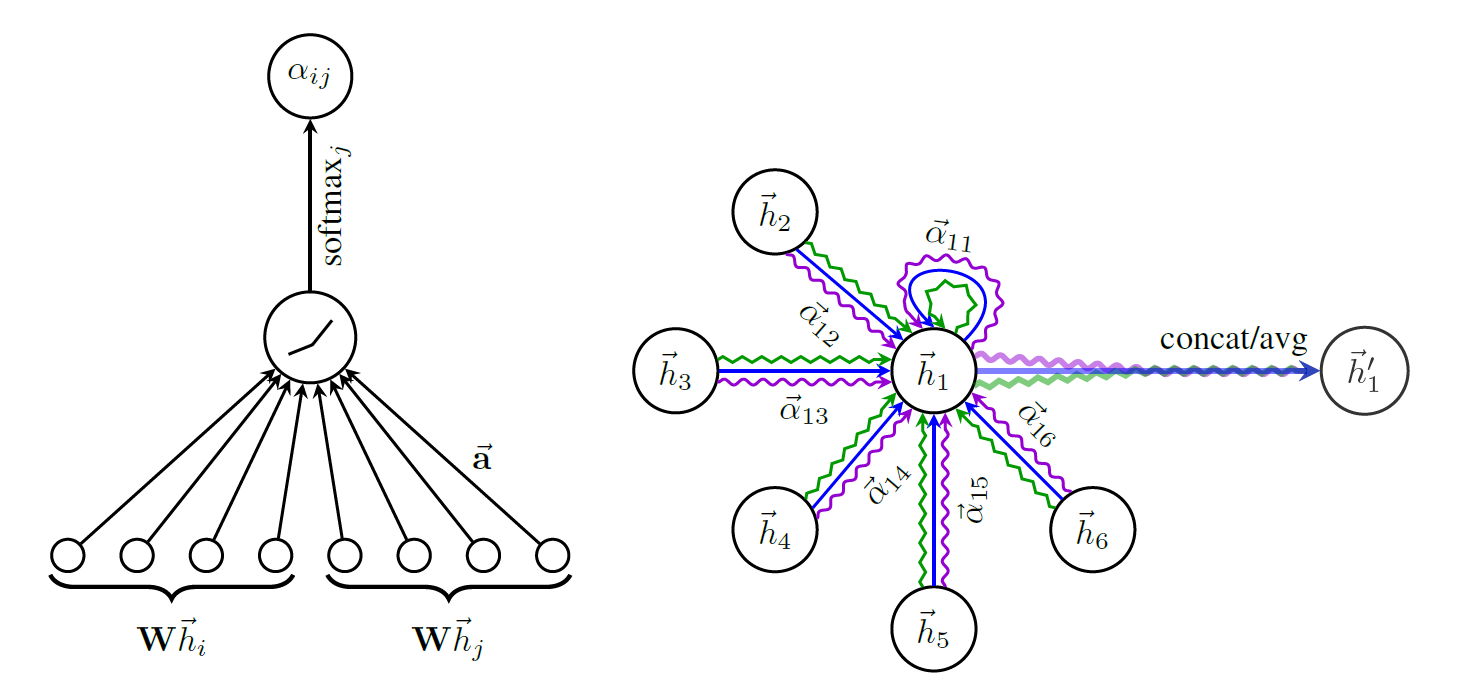
- (self-attention) self-attention coefficient $e_{ij}=a(\mathbf{W}\vec{h_i}, \mathbf{W}\vec{h_j})$: j번째 node가 i번째 node에 영향을 주는 정도
- 이 때, masked attention을 활용하여 first-order neighbor nodes (1-hop)에 대해서만 attention coefficient를 계산
- 하나의 노드가 다른 모든 노드들로부터 받는 영향을 파악하기 때문에 그래프의 구조를 고려하지 않아도 됨. (이웃 노드의 정보)
- 다른 node들과 비교하기 위해 normalize를 진행 (softmax): $\alpha_{ij}=softmax_j(e_{ij})=\frac{exp(e_{ij})}{\sum_{k \in \mathcal{N}}exp(e_{ik})}$
- (In this study) attention mechanism $a$로 $\vec{\mathbf{a}} \in \mathbb{R}^{2F’}$ single-layer feedfoward neural network + LeakyReLU 적용
- \[\alpha_{ij}=softmax_j(LeakyReLU(a(\mathbf{W}\vec{h_i}, \mathbf{W}\vec{h_j})) =\frac{exp(LeakyReLU(\vec{\mathbf{a}}^T[\mathbf{W}\vec{h_i}||\mathbf{W}\vec{h_j}]))}{\sum_{k \in \mathcal{N}}exp(LeakyReLU(\vec{\mathbf{a}}^T[\mathbf{W}\vec{h_i}||\mathbf{W}\vec{h_k}]))}\]
- (features) linear combination을 적용하여 각 node에 대한 features로 사용 → multi-head attention을 concat
- \(\vec{h'_i} = \Vert_{k=1}^K \sigma(\sum_{j \in \mathcal{N}_i}\alpha_{ij}^k\mathbf{W}^k\vec{h_j})\) where k: attention 번호
- (final layer) multi-head attention 결과에 대해 평균을 내서 결과 산출
- \[\vec{h_i'} = \sigma(\frac{1}{K}\sum_{k=1}^K\sum_{j \in \mathcal{N}_i}\alpha_{ij}^k\mathbf{W}^k\vec{h_j})\]
2.2. Comparisons to Related Work
- 효율성: node-node (edge) 단위로 계산할 수 있어 병렬처리 가능 + multi-head 계산 시에도 concat만 하므로 각 head 단위에서 독립적으로 병렬계산 가능 → GCN과 동등한 정도의 complexity
- 해석 가능성: different importances를 줄 수 있어 해석 용이
- 확장성
- 전체 그래프 구조(direct 여부 등)가 달라도 동일한 attention mechanism을 사용, inductive learning 가능 (unseen graph에 대해 적용 가능)
- 이웃 수와 순서를 고려하지 않음
- 노드의 구조보다는 노드의 feature를 통해 산출하여 그래프 구조를 몰라도 사용 가능
- Future works
- the tensor manipulation framework we used only supports sparse matrix multiplication for rank-2 tensors, which limits the batching capabilities of the layer as it is currently implemented (especially for datasets with multiple graphs).
- Depending on the regularity of the graph structure in place, GPUs may not be able to offer major performance benefits compared to CPUs in these sparse scenarios.
- It should also be noted that the size of the “receptive field” of our model is upper-bounded by the depth of the network (similarly as for GCN and similar models). Techniques such as skip connections (He et al., 2016) could be readily applied for appropriately extending the depth, however.
- parallelization across all the graph edges, especially in a distributed manner, may involve a lot of redundant computation, as the neighborhoods will often highly overlap in graphs of interest.
3 Evaluation
- Transductive learning / Inductive learning을 구분하여 수행
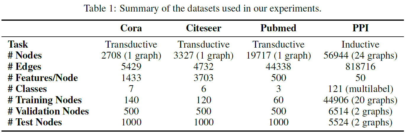
3.1. Datasets
3.2. State-of-the-art Methods
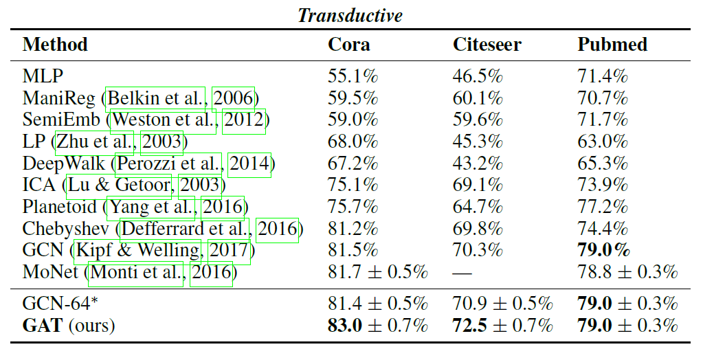
- Transductive learning: Label Propagation, SemiEmb, ManiReg, Deep-Walk, ICA, Planetoid, GCNs
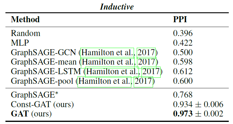
- Inductive learning: GraphSAGE, GraphSAGE-GCN, GraphSAGE-mean, GraphSAGE-LSTM, GraphSAGE-pool
3.3. Experimental Setup
- (Transductive learning) For the transductive learning tasks, we apply a two-layer GAT model. Its architectural hyperparameters have been optimized on the Cora dataset and are then reused for Cite-seer. The first layer consists of K = 8 attention heads computing F’ = 8 features each (for a total of 64 features), followed by an exponential linear unit (ELU) nonlinearity. The second layer is used for classification: a single attention head that computes C features (where C is the number of classes), followed by a softmax activation. For coping with the small training set sizes, regularization is liberally applied within the model. During training, we apply L2 regulariza-tion with λ = 0.0005. Furthermore, dropout (Srivastava et al., 2014) with p = 0.6 is applied to both layers’ inputs, as well as to the normalized attention coefficients (critically, this means that at each training iteration, each node is exposed to a stochastically sampled neighborhood). Similarly as observed by Monti et al. (2016), we found that Pubmed’s training set size (60 examples) required slight changes to the GAT architecture: we have applied K = 8 output attention heads (instead of one), and strengthened the L2 regularization to λ = 0.001. Otherwise, the architecture matches the one used for Cora and Citeseer.
- (Inductive learning) For the inductive learning task, we apply a three-layer GAT model. Both of the first two layers consist of K = 4 attention heads computing F’ = 256 features (for a total of 1024 features), followed by an ELU nonlinearity. The final layer is used for (multi-label) classification: K = 6 attention heads computing 121 features each, that are averaged and followed by a logistic sigmoid activation. The training sets for this task are sufficiently large and we found no need to apply L2 regularization or dropout—we have, however, successfully employed skip connections (He et al., 2016) across the intermediate attentional layer. We utilize a batch size of 2 graphs during training. To strictly evaluate the benefits of applying an attention mechanism in this setting (i.e. comparing with a near GCN-equivalent model), we also provide the results when a constant attention mechanism, a(x, y) = 1, is used, with the same architecture—this will assign the same weight to every neighbor.
- Both models are initialized using Glorot initialization (Glorot & Bengio, 2010) and trained to mini-mize cross-entropy on the training nodes using the Adam SGD optimizer (Kingma & Ba, 2014) with an initial learning rate of 0.01 for Pubmed, and 0.005 for all other datasets. In both cases we use an early stopping strategy on both the cross-entropy loss and accuracy (transductive) or micro-F1 (inductive) score on the validation nodes, with a patience of 100 epochs1.
3.4. Results
4 Conclusions
We have presented graph attention networks (GATs), novel convolution-style neural networks that operate on graph-structured data, leveraging masked self-attentional layers. The graph attentional layer utilized throughout these networks is computationally efficient (does not require costly matrix operations, and is parallelizable across all nodes in the graph), allows for (implicitly) assigning different importances to different nodes within a neighborhood while dealing with different sized neighborhoods, and does not depend on knowing the entire graph structure upfront—thus addressing many of the theoretical issues with previous spectral-based approaches. Our models leveraging attention have successfully achieved or matched state-of-the-art performance across four well-established node classification benchmarks, both transductive and inductive (especially, with completely unseen graphs used for testing). There are several potential improvements and extensions to graph attention networks that could be addressed as future work, such as overcoming the practical problems described in subsection 2.2 to be able to handle larger batch sizes. A particularly interesting research direction would be taking advantage of the attention mechanism to perform a thorough analysis on the model interpretability. Moreover, extending the method to perform graph classification instead of node classification would also be relevant from the application perspective. Finally, extending the model to incorporate edge features (possibly indicating relationship among nodes) would allow us to tackle a larger variety of problems.
- 참고
-
Attention and Self-attention: 어텐션 메커니즘과 transfomer(self-attention)
-
Attention과 문장 길이 문제 해결: 신경망 번역 모델의 진화 과정
-
Attention, GNN, GAT의 발전 과정: [DMQA Open Seminar] Graph Attention Networks
-
댓글남기기