[논문리뷰] Visualizing and Understanding Convolutional Networks

Visualizing and Understanding Convolutional Networks는 기존의 CNN 모델의 동작 방식에 대해 시각화를 통해 접근하였습니다. 왜 학습이 잘 되는지, 어떻게 학습이 진행되는지에 대해 Deconvolution 개념을 도입하여 시각화 분석을 하였으며, AlexNet보다 성능이 향상된 모델을 제시합니다. (문법적인 오류가 있을 수 있습니다.)

Abstract

Large Convolutional Network models have recently demonstrated impressive classification performance on the ImageNet benchmark Krizhevsky et al. [18]. However there is no clear understanding of why they perform so well, or how they might be improved. In this paper we explore both issues. We introduce a novel visualization technique that gives insight into the function of intermediate feature layers and the operation of the classifier. Used in a diagnostic role, these visualizations allow us to find model architectures that outperform Krizhevsky et al. on the ImageNet classification benchmark. We also perform an ablation study to discover the performance contribution from different model layers. We show our ImageNet model generalizes well to other datasets: when the softmax classifier is retrained, it convincingly beats the current state-of-the-art results on Caltech-101 and Caltech-256 datasets.

1. Introduction

• There is little understanding of internal operation of complex convolutional network models and how they achieve good performance.
• Therefore, the paper introduces technique that reveals which input stimuli excites feature maps.
• By this, we can also observe how the features evolve during training, and diagnose the potential problems.
• In addition, the authors performed sensitivity analysis by revealing the important scene for classification.

1.1. Related Work

• Visualization: The studies about visualizing features are limited to the first layer based on projections to pixel space. In higher layers, invariances of units are too complex that simple quadratic approximation is not enough to capture. Therefore, this paper provides non-parametric approach by showing the patterns that activate feature map.
  • Simonyan et al. projected back from fully connected layers. → This paper uses convolutional layers.
  • Girshick et al. identifies patches that strongly activate at higher layers. (just crops of input images) → This paper use top-down projections within each patch.
• Feature Generalization: generalization ability of convnet features is also explored by Donahue et al. and Girshick et al.

2. Approach

• The paper uses standard fully supervised convnet models, which capture 2D image to C classes through series of layers.
  • Each layer consists of (1) convolution of the previous layer output (or, in the case of the 1st layer, the input image) with a set of learned filters; (2) passing the responses through ReLU function; (3) [optionally] max pooling over local neighborhoods and (4) [optionally] a local contrast operation that normalizes the responses across feature maps.

2.1. Visualization with a Deconvnet

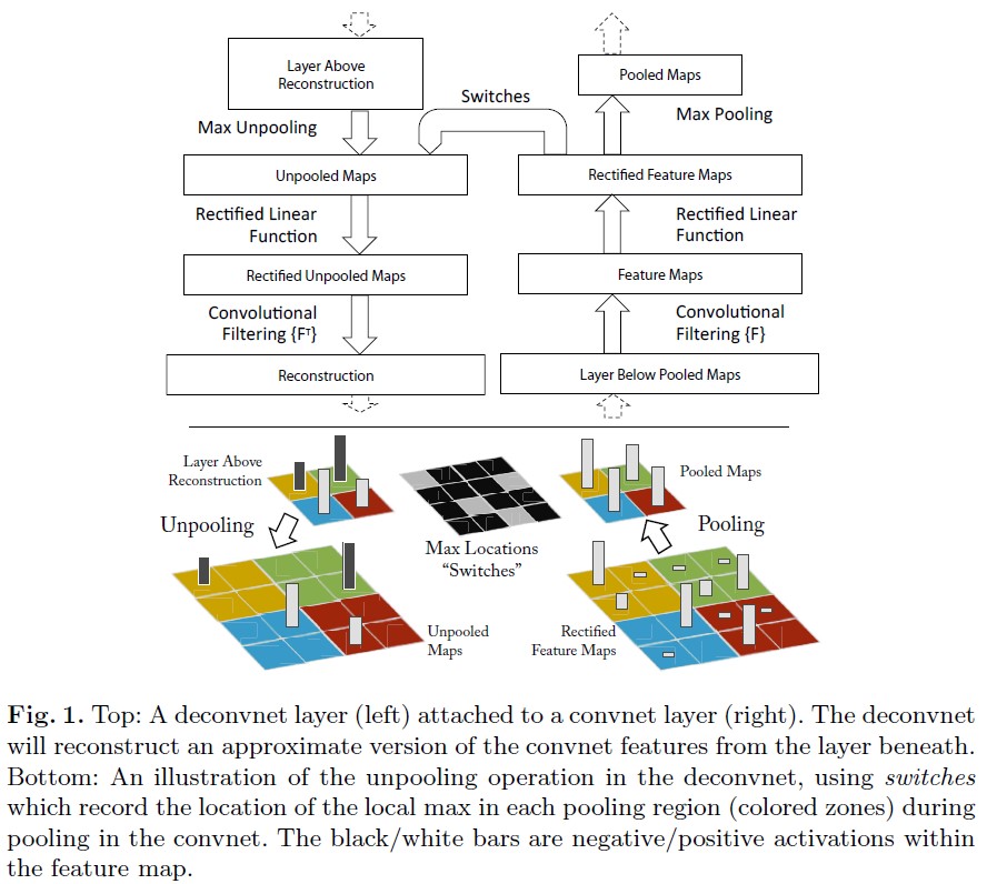
• In the paper, the authors perform Deconvolutional Network (deconvnet) to map feature activities back to input pixel space.
  • Deconvnet model uses the components of convnet (such as pooling and filtering) in reverse.
  • deconvnet is attached to each of convnet layers.
• Unpooling: The model records the locations of maxima for each pooling layer as switch variables. This way, deconvnet can preserve the structure of the stimulus and reconstruct the layer.
• Rectification: Through relu non-linearity, the model passes signal.
• Filtering: The model uses transpose of filters and applies to rectified maps. In this way, the filters are flipped horizontally and vertically.
• By these approaches, the model can get the weighted structure according to their contributions.
• Since there is no generative process, the projections are not samples. Therefore, the process is like backpropping a single strong activation, with independently imposed ReLU and no contrast normalization.

3. Training Details

• The architecture is similar to model of Krizhevsky et al., with one difference that this papaer uses dense connections instead of sparse connections for 2 GPUs (This paper uses one GPU).
• The images from ImageNet 2012 training set were preprocessed by resizing, cropping (256256), subtracting mean, and 10 different sub-crops with size 224224.
• They used SGD with batch size 128 and learning rate 0.01, momentum 0.9. Dropout layer with rate 0.5 is also used in fully connected layers.
• To visualize the first layer filters, each filter was renormalized if the RMS value exceeds a radius of 0.1.
• To boost training set size, different flips and crops are used.
• The training was stopped after 70 epochs.

4. Convnet Visualization

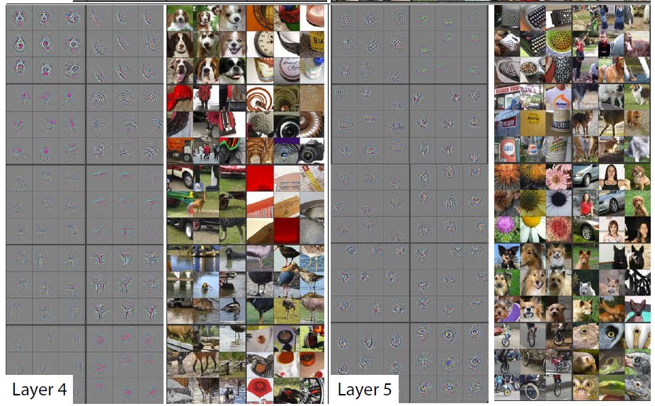
• Feature Visualization: Top 9 activations are shown for a given feature map. Each activation is projected seperately and reveals different structures to excite map and invariance to input deformations.

  

• Feature Evolution during Training: The lower layers are converged in few epochs. On the other hand, upper layers need more epochs to be fully converged.

4.1. Architecture Selection

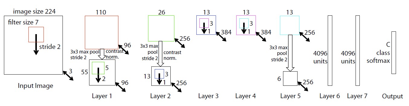
• When visualize the layers, we can capture some problems of the architecture.
  • The first layer had little coverage of mid frequencies (only extremely high or low frequency information)
  • Due to large stride (4), the second layer shows aliasing artifacts.
• To deal with the problems, filter size of first layer was reduced to 77 (from 1111); and stride was reduced to 2.

4.2. Occlusion Sensitivity

• To clarify the image classification process that whether the model truly identifies the location of object (or just uses surrounding context), they occlude some portions of input as grey square.
  • The probability of correct class dropped largely.
• The paper showed that the visualization corresponds to the image structure that stimulates that feature map (validating the other visualizations).

5. Experiments

5.1. ImageNet 2012

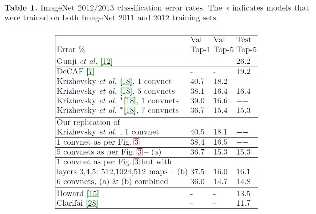
• This model outperformed the architecture of Krizhevsky et al.

  

• Varying ImageNet Model Sizes:

  

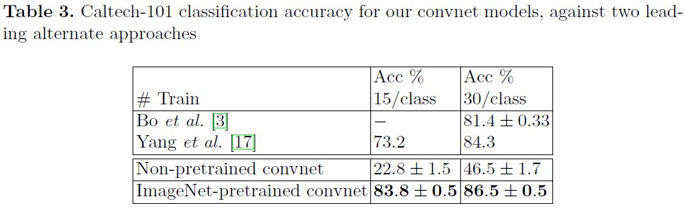
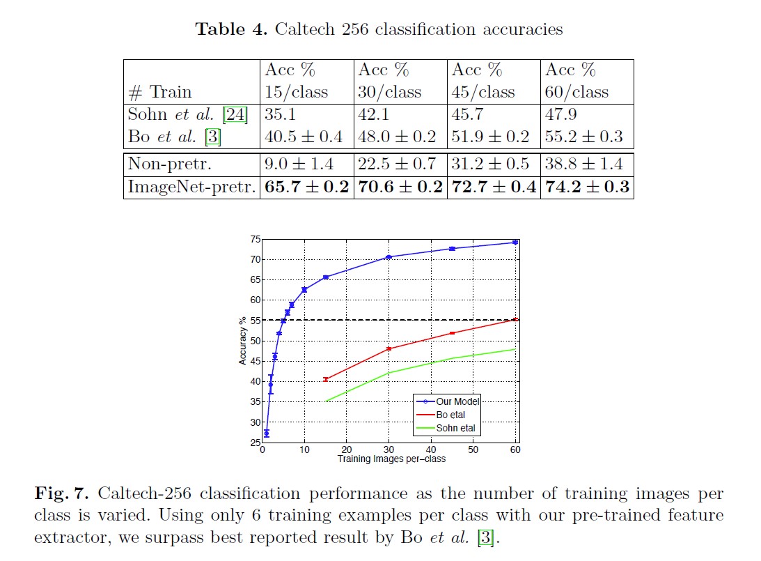
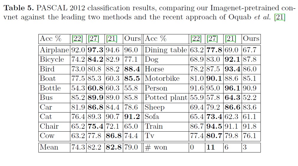
5.2. Feature Generalization

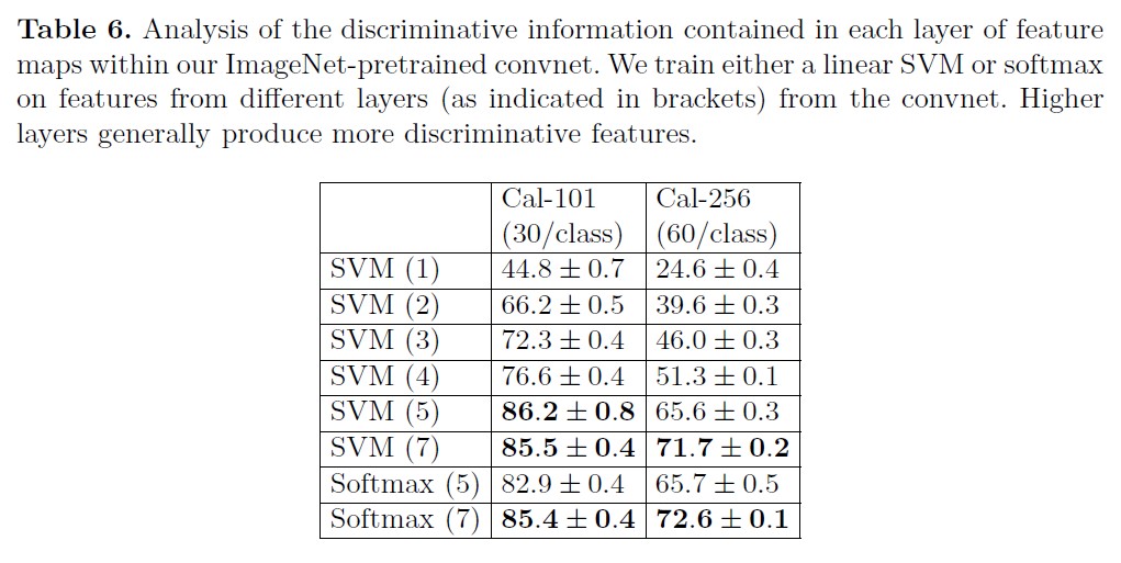
5.2. Feature Analysis

6. Discussion

• We explored large convolutional neural network models, trained for image classification, in a number of ways. First, we presented a novel way to visualize the activity within the model. This reveals the features to be far from random, uninterpretable patterns. Rather, they show many intuitively desirable properties such as compositionality, increasing invariance and class discrimination as we ascend the layers. We also show how these visualization can be used to identify problems with the model and so obtain better results, for example improving on Krizhevsky et al. ’s [18] impressive ImageNet 2012 result. We then demonstrated through a series of occlusion experiments that the model, while trained for classification, is highly sensitive to local structure in the image and is not just using broad scene context. An ablation study on the model revealed that having a minimum depth to the network, rather than any individual section, is vital to the model’s performance.
• Finally, we showed how the ImageNet trained model can generalize well to other datasets. For Caltech-101 and Caltech-256, the datasets are similar enough that we can beat the best reported results, in the latter case by a significant margin. Our convnet model generalized less well to the PASCAL data, perhaps suffering from dataset bias [25], although it was still within 3.2% of the best reported result, despite no tuning for the task. For example, our performance might improve if a different loss function was used that permitted multiple objects per image. This would naturally enable the networks to tackle the object detection as well.

---

• 제 개인 Notion에서도 확인 가능합니다.