[ML] Explainable AI

Towardsdatascience
해당 글은 데이터 기반의 솔루션을 제시할 때 explanation이 필요하다는 관점에서 제시한 방법들이다. 위의 글들을 번역 및 정리한 내용이다.
아직까지 대부분의 기업에서는 데이터를 기반으로 추론하는 것이, 오랜 경험자나 전문가의 노하우와 감보다 영향력이 없다고 한다. 따라서 어떠한 결과가 어떻게 나왔는지에 대한 해석이 되어야 그 분석이 유의미해질 것이라 생각한다.

Explainable AI는 두 가지로 구분할 수 있다.
- Intrinsically interpretable predictive model (i.e. rule-based)
- Post-hoc interpretable model (black-box model)
Post-hoc interpretable model은 다시 두 가지로 구분된다.
- Global models (describe average behavior of the model)
- Local models (explain individual predictions)
대부분의 Post-hoc interpretable model은 model-agnostic하다. (알고리즘과 상관없이 독립적으로 계산이 가능하다.)

일반적으로는 local 모델이 global 모델보다 자주 사용된다.

model	category	characteristic
LIME	local	model-agnostic
SHAP	local	model-agnostic
PDP	global	model-agnostic
ICE	local	model-agnostic
ALE	global	model-agnostic

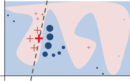
LIME (Local Interpretable Model-Agnostic Explanations)

local explanation을 제공한다. 즉, 특정 데이터가 특정 클래스로 분류된 이유 등 개별 point에 집중한다.
어떠한 모델으로 분석을 진행하는지에 상관없이, linear model을 사용하여 해석을 제공한다.
- linear model은 복잡한 데이터 혹은 모델은 설명하지 못할 수 있지만, local observation에 한해서는 적절한 설명을 제공할 것이다. → 관련 내용은 이 논문에서 더 자세히 확인할 수 있다.
  
  The main concept around LIME is that even though linear models won’t be able to explain well complex data/model, when trying to explain an observation locally it can provide an adequate explanation
원래 데이터 셋을 사용하여 설명하고자 하는 관찰값 주변의 데이터들을 샘플링하는 방식을 사용한다. (perturbed samples)
- 따라서 Categorical feature를 포함하고 있다면, one-hot-encoding 보다는 정수 형태의 label을 사용하는 것을 권장한다. 이와 관련해서는 github와 강의를 참고할 수 있다.
- 샘플링된 관찰값과 실제 관찰값의 유사도에 따라 가중치가 부여된다.
LIME은 어떤 데이터를 사용하는지에 따라 세 가지 explainers를 사용한다: tabular explainer, image explainer, text explainer

LIME은 실행 속도가 빠르고(특히, tabular explainer의 경우), 작동 방식이 매우 직관적이다. 그러나 전처리가 필요하다.

Examples

가장 먼저, 분석의 목적(regression / classification)과 그에 따른 explainer을 설정한다.

  from lime.lime_tabular import LimeTabularExplainer
  lime_explainer = LimeTabularExplainer(train_data.values, 
  mode = ’classification’, feature_names = new_feature_names, class_names = [‘Deny’, ’Approve’], verbose=True, 
  random_state = 42)

1) 어떤 변수에 대해 해석을 하고자 하는지, 2) 확률분포를 생성하는 모델이 무엇인지 (ex classification의 경우 predict_proba) 3) local linear model을 생성하기 위한 최대 feature 개수 (default 10)
```
  exp = lime_explainer.explain_instance(instance, trained_model.predict_proba)
  exp.show_in_notebook(show_table=True)
```
결과에 대한 해석은 다음과 같다.
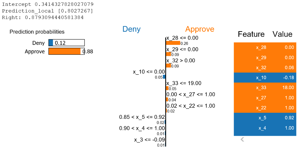
- 왼쪽 상단에는 intercept, local prediction, true prediction을 볼 수 있으며, 각 class에 속하는 확률을 알 수 있다. (앞서 언급하였듯, 개별 point에 대한 해석을 진행하고자 할 때 사용한다.)
- 오른쪽에는 각 feature의 값들을 볼 수 있다. 주황색은 approve class에 기여한 features, 파란색은 deny에 기여한 features이며, 큰 영향을 미친 feature 순으로 나열된다.
- print(‘R²: ‘+str(exp.score))으로 local model의 설명력도 확인이 가능하다. 해당 값을 확인하여 이 해석을 신뢰할 지 결정할 수 있다.
- exp.local_exp을 통해 각 feature별 weight(coefficient)를 확인할 수 있다.

SHAP (SHapley Additive exPlanations)

SHAP는 각 feature가 예측에 얼마나 기여하는지를 설명한다.
coalitional game theory의 Shapley value를 기반으로 나온 해석 방법이다.
- 게임 이론에서는, 어떤 그룹이 게임에서 이겼을 때, 각 참가자가 기여한 정도에 따라 payout을 나눠가지는 방법을 설명한다.
특정 feature의 기여도를 계산하는 방법은, 해당 feature를 포함하지 않는 모든 조합에 대하여, 그 feature를 추가한 경우과 하지 않은 경우 예측력의 차이를 구하고, 각 조합에 대해 예측력 평균을 구하는 것이다.
계산에 소요되는 비용이 크고, 해당 feature가 빠질 경우 완전히 새로운 모델이 될 수 있으므로 (Adi Watzman 강의 참고), approximations와 optimizers를 사용하여 이 문제를 보완하고자 한다.
- KernalSHAP(LIME과 유사), TreeSHAP(tree-based), DeepSHAP(deep learning model에서 빠르게 approximation)
SHAP은 간편하게 사용할 수 있으며, feature들에 대한 overall view를 제공한다. 또한 approximation이 아닌 정확한 값을 계산할 수 있다. 그러나 직관적인 해석이 어려운 편이다.

Examples

해당 글에서는 TreeSHAP에 대한 예시를 제공했다.

여기서도 가장먼저 explanier을 정의한다.

  import shap
  shap.initjs() #This is for us to be able to see the visualizations 
  explainer = shap.TreeExplainer(trained_model)

classification의 경우 SHAP value는 두 클래스에 대해 모두 산출이 되며, 어떠한 클래스를 index로 사용할지 결정해야 한다. (해당 글에서는 class 1을 reference로 설정하였다)
```
  shap_values = explainer.shap_values(instance)
  shap.force_plot(base_value=explainer.expected_value[1], shap_values[1], features=instance, feature_names=new_feature_names)
```
결과는 다음과 같다.
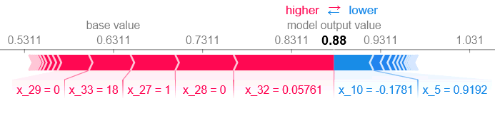
- 볼드체로 표시된 값이 prediction이며, 왼쪽부터 feature별로 training set의 average of predictions이 표시된다. 각 변수의 기여도를 더하고 빼서 해당 값으로 수렴한다. (빨간색: class 1에 기여, 파란색: class 0에 기여) 또한, 기여 정도에 따라 정렬되어 있다.
- Explainer.expected_value[1] + sum(shap_values[1])을 통해 approximation이 아닌 정확한 prediction 값을 확인할 수 있다.
class에 따른 feature의 behavior을 확인할 수도 있다. 이를 위해 가장 먼저, test set에 대해 SHAP vlaue를 계산한다.
```
  test_shap_values = explainer.shap_values(test_data.values)
  shap.summary_plot(shap_values[1], test_data.values)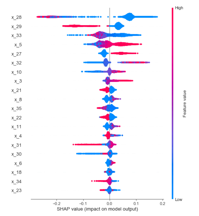
```
- x축은 prediction에 대한 기여도를, y축(좌)은 가장 영향력 있는 feature의 순으로 정렬이 된다.
- 오른쪽의 y축은 각 feature에 대해 원래의 값을 어떻게 해석해야하는지 나타낸다. 예를 들어, 파란색은 feature의 값이 작음을, 빨간색은 feature의 값이 큰 것을 나타낸다.
다른 시각화 방법은 Github에서 확인할 수 있다.

InterpretML

glassbox 모델, 예를 들어 linear regression, logistic regression, decision trees 모델에 대해 InterpreML을 통해 model-specific explainable tool (global/local explanations)을 제공할 수 있다.
- blackbox 모형의 경우, 앞서 언급된 LIME, Kernel SHAP 등 model-agnostic explainability tool (local explanations)을 사용한다.
InterpretML은 local/global context가 설명 가능한 Boosting Machine Package이다.
- glassbox 모형에 대한
- scikit-learn과 호환가능하여, 동일한 hyperparameter로 튜닝이 가능하다.
- Microsoft Researchers가 개발한 Explainable Boosting Machine (EBM) model을 포함하고 있다.

Explainable Boosting Machine (EBM)

glassbox model으로, Random Forest나 Boosted Trees와 유사한 성능을 보인다.
linear model과 유사하게 Generalized Additive Model (GAM)이다.
- linear model은 $Y=\beta_0+\beta_1x_1+…+\beta_nx_n$의 식으로 구성
- GAM은 $Y=\beta_0+f(x_1)+…+f(x_n)$의 식으로 구성 (f 함수는 특정 point의 기여도를 나타낸다고 할 수 있다.)
EBM은 GAM을 개선한 모델으로, bagging이나 boosting을 통해 feature function을 학습한다.
- 반복을 많이 하게 되면 다중공선성의 영향을 완화하여 학습이 더 잘 되도록 한다.
- 각 반복마다 하나의 feature만을 사용한 작은 트리들이 순차적으로 구성된다. boosting 과정에서 잔차(residual)이 업데이트 되며 다른 feature에 대한 새로운 트리들이 생겨난다. 매 반복마다 각 feature에 대해 동일한 과정이 수행된다. 이후, 각 feature에 대해 생성된 트리들을 통해 예측값에 미치는 기여도를 확인한다.
또한 pairwise interaction term을 자동으로 감지하여 정확도를 높일 수 있다.

Examples

Kaggle의 heart failure prediction dataset을 사용하였다.
EBM과 Logistic regression을 사용하면 log odds를 통해 각 feature의 기여 정도를 확인할 수 있다.

1. EBM (glassbox)

Global explanation을 확인하려면 다음과 같이 실행한다.
```
  ebm_global = trained_ebm.explain_global()
  show(ebm_global)
```
- 각 feature들에 대한 전반적인 중요도는 트레이닝셋의 각 feature들에 대한 예측값들의 평균이다. (앞서 언급하였듯, 한 번에 하나의 feature을 사용하여 점수를 계산하기 때문)
- 위 이미지에서 회색으로 표시된 구간은 error bars로, 특정 구간에서의 uncertainty를 의미한다. (trained_ebm.term_standard_deviations_[4]로 특정 feature에 대한 error bar 크기를 확인가능하다.)

Local explanation은 다음과 같이 확인한다.

  ebm_local = trained_ebm.explain_local(X_test[10:15], y_test[10:15])
  show(ebm_local)

2. Logistic Regression (glassbox)

Global explanation을 확인한다.
```
  lr_global = trained_lr.explain_global()
  show(lr_global)
```
- EBM과는 달리, 크기와 부호를 모두 제공한다.
Local explanation을 확인한다.

3. LightGBM w. LIME and SHAP (blackbox)

LightGBM은 결측치가 존재하여도 학습이 가능하다.

InterpretML package는 blackbox 모델에 대해서는 위와 같은 설명을 제공하지 않기 때문에 LIME과 SHAP를 활용하였다.

InterpretML은 KernalSHAP 함수를 제공하므로 이를 사용하였다.

  from interpret.blackbox import ShapKernel
  shap = ShapKernel(predict_fn=trained_LGBM.predict_proba, data=X_train)
  shap_local = shap.explain_local(X_test[10:15], y_test[10:15])
  show(shap_local)

LIME을 사용한 결과는 다음과 같다.

  lime = LimeTabular(predict_fn=trained_LGBM.predict_proba, data=X_train)
  lime_local = lime.explain_local(X_test[10:15], y_test[10:15])
  show(lime_local)

추가로, InterpretML은 plotly를 활용한 EDA 역시 제공한다.

  from interpret import show
  from interpret.provider import InlineProvider
  from interpret import set_visualize_provider
  set_visualize_provider(InlineProvider())
  from interpret.data import ClassHistogram
  hist = ClassHistogram().explain_data(X_train, y_train, name="Train Data")
  show(hist)

xai

하이퍼파라미터 튜닝 시 ROC 커브를 비교할 때도 사용할 수 있다.

  from interpret.glassbox import ExplainableBoostingClassifier
  from sklearn.model_selection import RandomizedSearchCV
  param_test = {'learning_rate': [0.001,0.005,0.01,0.03],
                'interactions': [5,10,15],
                'max_interaction_bins': [10,15,20],
                'max_rounds': [5000,10000,15000,20000],
                'min_samples_leaf': [2,3,5],
                'max_leaves': [3,5,10]}
  n_HP_points_to_test=10
  LGBM_clf = LGBMClassifier(random_state=314, n_jobs=-1)
  LGBM_gs = RandomizedSearchCV(
      estimator=LGBM_clf,
      param_distributions=param_test,
      n_iter=n_HP_points_to_test,
      scoring="roc_auc",
      cv=3,
      refit=True,
      random_state=314,
      verbose=False,
  )
  LGBM_gs.fit(X_train, y_train)
    
  from interpret import perf
  roc = perf.ROC(gs.best_estimator_.predict_proba, feature_names=X_train.columns)
  roc_explanation = roc.explain_perf(X_test, y_test)
  show(roc_explanation)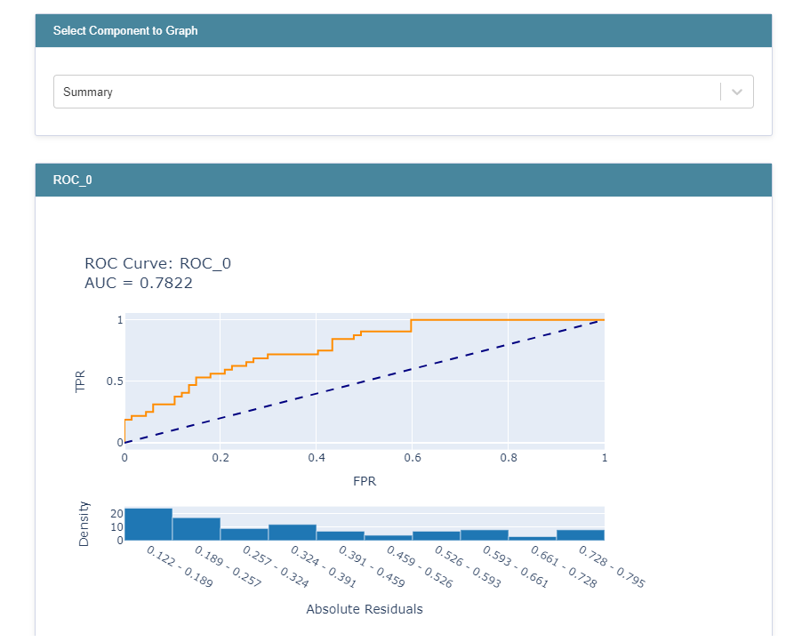

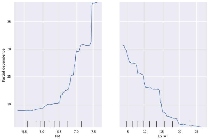
xai

Partial Dependence Plot (PDP)

global, model-agnostic 방법이다.
numeric과 categorical values에 모두 사용할 수 있다.
계산 과정은 다음과 같다.
- 먼저, 특정 변수와 그 변수에 대한 grid 값들을 선정한다.
- 특정 변수의 값들을 grid 값들로 대체한 후 그 값들마다 예측값의 평균을 계산한다.
- 이를 curve로 그려낸다.
3차원 이상을 해석하기는 어려우므로, 두 변수들에 대한 PDP를 그려서 확인한다.
scikit-learn의 [plot_partial_dependence 함수](https://scikit-learn.org/stable/modules/generated/sklearn.inspection.plot_partial_dependence.html)를 사용하여 확인할 수 있다.
두 변수가 높은 correlation을 가질 경우 bias를 다 표현할 수 없기 때문에 다음의 ALE를 권장한다.

Individual Conditional Expectation (ICE)

local, model-agnostic 방법이다.
PDP와 유사하지만, 평균적인 기여도를 표현하기보다는, 데이터들의 기여도를 각각 표현한다.
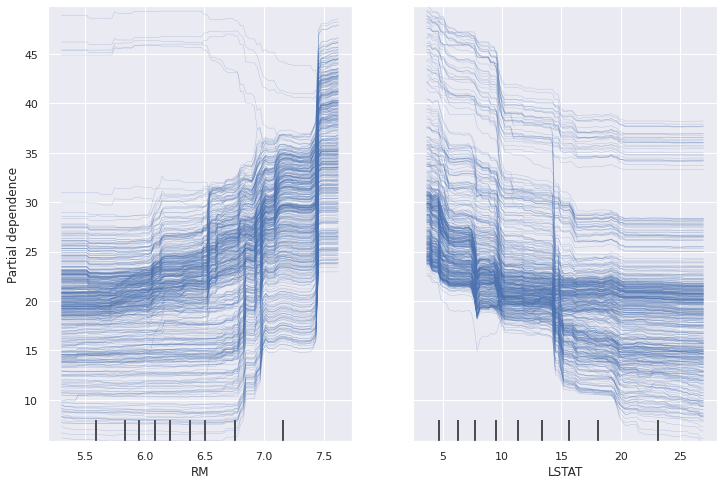
- 하나의 선이 하나의 데이터를 설명하므로, 타 데이터들과 다른 경향을 띄는 데이터들을 확인할 수 있다.
너무 많은 데이터가 존재할 때 해석이 어려워질 수 있다.

Accumulated Local Effects (ALE)

global, model-agnostic 방법을 사용한다.
PDP의 alternative로 사용된다.
- bias를 표현하기 위해, 특정 변수에 대해 모든 행들에 동일한 값을 대체하기 보다는, 해당 값의 유사한 값들(windows)으로 대체한다.
- 그 후 예측값의 평균을 내어 M-plot을 그린다.
그러나 모든 상관된 (correlated) 변수들에 대해 combinded effect를 나타내는 것은 동일하다.
- 실제로 변수A는 예측값에 영향을 미치고 (A→예측값), 변수B는 그렇지 않더라도(B!→예측값), 변수A와 변수B의 상관관계가 높을 경우 이 두 변수가 모두 예측값에 영향을 미친다고 설명할 것이다.
ALE는 windows에 대한 평균이 아니라, empirical quantiles를 사용하여 windows별 예측값들 간 차이를 계산한다.
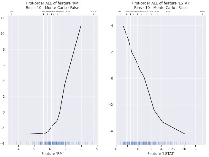
- 위의 이미지에서는, 전체의 10%씩 특정 window 값을 갖도록 하였다. 그러나, 이를 설정하는 방법에 대해서는 아직 결정된 게 없다.
해당 패키지는 깃헙에서 확인이 가능하다.

향후 더 참고하고자 하는 글
- [ML] Explainable AI - Shapley Value
- Interpretable machine learning

Twitter Facebook LinkedIn

전은지

[ML] Explainable AI

LIME (Local Interpretable Model-Agnostic Explanations)

Examples

SHAP (SHapley Additive exPlanations)

Examples

InterpretML

Explainable Boosting Machine (EBM)

Examples

1. EBM (glassbox)

2. Logistic Regression (glassbox)

3. LightGBM w. LIME and SHAP (blackbox)

Partial Dependence Plot (PDP)

Individual Conditional Expectation (ICE)

Accumulated Local Effects (ALE)

공유하기

댓글남기기

참고

[논문리뷰] XL-Net: Generalized Autoregressive Pretraining for Language Understanding

[논문리뷰] Graph Heterogeneous Multi-Relational Recommendation (GHCF)

[논문리뷰] Modeling Relational Data with Graph Convolutional Networks (RGCN)

[논문리뷰] K-BERT: Enabling Language Representation with Knowledge Graph